Classical Mechanics: Double Pendulum Dynamics & Chaos - Small-Angle Normal Modes, Resonance & Harmonic Beats • Interactive Visualization

Simulation 1

Small-Angle Normal Modes, Resonance & Harmonic Beats

Python 3.11 with Matplotlib Slider Ready

"""
Coupled Harmonic Normal Modes, Eigenfrequencies & Beat Superposition
Small-Angle Linear Approximation of the Double Pendulum
Powered by Pyodide with Matplotlib Interactive Sliders
"""
import numpy as np
import matplotlib.pyplot as plt
from matplotlib.widgets import Slider

# Create 2-panel figure
fig = plt.figure(figsize=(10.5, 5.8))
gs = fig.add_gridspec(1, 2, width_ratios=[1.0, 1.2], wspace=0.28)
ax_pend = fig.add_subplot(gs[0, 0])
ax_beats = fig.add_subplot(gs[0, 1])
plt.subplots_adjust(bottom=0.30, top=0.90, left=0.09, right=0.94)

# Sliders
ax_mratio = plt.axes([0.15, 0.16, 0.32, 0.024])
ax_lratio = plt.axes([0.15, 0.06, 0.32, 0.024])
ax_mode   = plt.axes([0.62, 0.16, 0.32, 0.024])
ax_amp    = plt.axes([0.62, 0.06, 0.32, 0.024])

s_mratio = Slider(ax_mratio, 'm2/m1 Ratio', 0.1, 4.0, valinit=1.0, valstep=0.1)
s_lratio = Slider(ax_lratio, 'L2/L1 Ratio', 0.2, 3.0, valinit=1.0, valstep=0.05)
s_mode   = Slider(ax_mode, 'Mode Mixture', -1.0, 1.0, valinit=0.0, valstep=0.05)
s_amp    = Slider(ax_amp, 'Amp θ0 (deg)', 1.0, 25.0, valinit=8.0, valstep=1.0)

def compute_normal_modes(mu, eta, mode_mix, theta0_deg, g=9.81, L1=1.0, t_max=18.0, steps=800):
    """
    mu  = m2 / m1
    eta = L2 / L1
    """
    th0 = np.radians(theta0_deg)
    L2 = eta * L1
    
    # Characteristic quadratic equation for omega^2:
    # det([ (1+mu)*L1*w^2 - (1+mu)*g,   mu*L2*w^2 ]
    #     [ L1*w^2,                    L2*w^2 - g ]) = 0
    #
    # (1+mu)*eta*(w^2)^2 - (1+mu)*(1+eta)*(g/L1)*w^2 + (1+mu)*(g/L1)^2 = 0
    # Divide by (1+mu): eta * W^2 - (1+eta)*W + 1 = 0  where W = w^2 * (L1/g)
    # Roots: W = [ (1+eta) +/- sqrt( (1+eta)^2 - 4*eta*(1 - ... ) ) ]
    
    A = eta
    B = -(1.0 + mu) * (1.0 + eta) * (g / L1)
    # Mass matrix M and Stiffness matrix K
    # M = [[ (1+mu)*L1^2, mu*L1*L2 ], [ mu*L1*L2, mu*L2^2 ]]
    # K = [[ (1+mu)*g*L1, 0        ], [ 0,         mu*g*L2 ]]
    M11 = (1.0 + mu) * L1**2
    M12 = mu * L1 * L2
    M22 = mu * L2**2
    K11 = (1.0 + mu) * g * L1
    K22 = mu * g * L2

# Solve generalized eigenvalues K v = w^2 M v
    # (K11 - w^2 M11)(K22 - w^2 M22) - (w^2 M12)^2 = 0
    # (M11*M22 - M12^2) (w^2)^2 - (K11*M22 + K22*M11) w^2 + K11*K22 = 0
    detM = M11 * M22 - M12**2
    trace_KM = K11 * M22 + K22 * M11
    detK = K11 * K22

disc = np.sqrt(max(0.0, trace_KM**2 - 4.0 * detM * detK))
    w1_sq = (trace_KM - disc) / (2.0 * detM)  # Lower frequency (In-phase)
    w2_sq = (trace_KM + disc) / (2.0 * detM)  # Higher frequency (Out-of-phase)

w1 = np.sqrt(max(0.01, w1_sq))
    w2 = np.sqrt(max(0.01, w2_sq))

# Eigenvector ratios r = theta2 / theta1
    # From 1st row: (K11 - w^2 M11) - w^2 M12 * r = 0  => r = (K11 - w^2 M11) / (w^2 M12)
    r1 = (K11 - w1_sq * M11) / (w1_sq * M12) # In-phase: r1 > 0
    r2 = (K11 - w2_sq * M11) / (w2_sq * M12) # Out-of-phase: r2 < 0

# Mode weights: mode_mix in [-1, 1]
    # +1 -> 100% Mode 1, -1 -> 100% Mode 2, 0 -> 50% Mode 1 + 50% Mode 2 (Beats)
    w_mode1 = 0.5 * (1.0 + mode_mix)
    w_mode2 = 0.5 * (1.0 - mode_mix)

t = np.linspace(0, t_max, steps)
    c1 = th0 * w_mode1
    c2 = th0 * w_mode2

th1_t = c1 * np.cos(w1 * t) + c2 * np.cos(w2 * t)
    th2_t = c1 * r1 * np.cos(w1 * t) + c2 * r2 * np.cos(w2 * t)

# Positions at t=0
    th1_now, th2_now = th1_t[0], th2_t[0]
    x1 = L1 * np.sin(th1_now); y1 = -L1 * np.cos(th1_now)
    x2 = x1 + L2 * np.sin(th2_now); y2 = y1 - L2 * np.cos(th2_now)

return t, th1_t, th2_t, w1, w2, r1, r2, x1, y1, x2, y2, L1, L2

t, th1_t, th2_t, w1, w2, r1, r2, x1, y1, x2, y2, L1, L2 = compute_normal_modes(
    s_mratio.val, s_lratio.val, s_mode.val, s_amp.val
)

# 1. Pendulum Display
line_arm, = ax_pend.plot([0, x1, x2], [0, y1, y2], 'o-', color='#10b981', lw=3, markersize=8)
bob1, = ax_pend.plot(x1, y1, 'o', color='#38bdf8', markersize=10)
bob2, = ax_pend.plot(x2, y2, 'o', color='#f59e0b', markersize=12)
ax_pend.plot(0, 0, 's', color='#f8fafc', markersize=6)
ax_pend.plot([0, 0], [0, -(L1 + L2 + 0.2)], color='#64748b', ls=':', lw=1.2)

R = L1 + L2 + 0.3
ax_pend.set_xlim(-R * 0.7, R * 0.7)
ax_pend.set_ylim(-R, 0.3)
ax_pend.set_aspect('equal')
ax_pend.set_title('Small-Angle Normal Mode Shape', fontsize=10.5, fontweight='bold', pad=6)
ax_pend.grid(True, linestyle=':', alpha=0.35)

# 2. Beat Superposition History
line_th1, = ax_beats.plot(t, np.degrees(th1_t), color='#38bdf8', lw=1.8, label=r'$\theta_1(t)$ Upper')
line_th2, = ax_beats.plot(t, np.degrees(th2_t), color='#f59e0b', lw=1.4, ls='--', label=r'$\theta_2(t)$ Lower')

# Beat envelope if both modes are active
if abs(s_mode.val) < 0.9:
    w_beat = abs(w2 - w1)
    env = np.degrees(np.radians(s_amp.val) * np.cos(0.5 * w_beat * t))
    line_env1, = ax_beats.plot(t, env, color='#94a3b8', ls=':', lw=1.2, alpha=0.7, label='Beat Envelope')
    line_env2, = ax_beats.plot(t, -env, color='#94a3b8', ls=':', lw=1.2, alpha=0.7)
else:
    line_env1, = ax_beats.plot(t, np.zeros_like(t), color='none')
    line_env2, = ax_beats.plot(t, np.zeros_like(t), color='none')

ax_beats.set_title(f'Harmonic Beats | ω1={w1:.2f} rad/s, ω2={w2:.2f} rad/s', fontsize=10.5, fontweight='bold', pad=6)
ax_beats.set_xlabel('Time $t$ (seconds)', fontsize=9)
ax_beats.set_ylabel('Deflection Angle (degrees)', fontsize=9)
ax_beats.grid(True, linestyle=':', alpha=0.35)
ax_beats.legend(loc='upper right', fontsize=7.5, framealpha=0.85)

def update(val):
    mu = s_mratio.val
    eta = s_lratio.val
    mix = s_mode.val
    amp = s_amp.val

t_n, th1_n, th2_n, w1_n, w2_n, r1_n, r2_n, x1_n, y1_n, x2_n, y2_n, L1_n, L2_n = compute_normal_modes(
        mu, eta, mix, amp
    )

line_arm.set_data([0, x1_n, x2_n], [0, y1_n, y2_n])
    bob1.set_data([x1_n], [y1_n])
    bob2.set_data([x2_n], [y2_n])

line_th1.set_ydata(np.degrees(th1_n))
    line_th2.set_ydata(np.degrees(th2_n))

if abs(mix) < 0.9:
        w_beat = abs(w2_n - w1_n)
        env_n = np.degrees(np.radians(amp) * np.cos(0.5 * w_beat * t_n))
        line_env1.set_data(t_n, env_n)
        line_env2.set_data(t_n, -env_n)
        line_env1.set_color('#94a3b8')
        line_env2.set_color('#94a3b8')
    else:
        line_env1.set_color('none')
        line_env2.set_color('none')

ax_beats.relim()
    ax_beats.autoscale_view(scalex=False, scaley=True)
    ax_beats.set_title(f'Harmonic Beats | ω1={w1_n:.2f} rad/s (r1={r1_n:+.2f}), ω2={w2_n:.2f} rad/s (r2={r2_n:+.2f})', fontsize=10.0, fontweight='bold', pad=6)

fig.canvas.draw_idle()

s_mratio.on_changed(update)
s_lratio.on_changed(update)
s_mode.on_changed(update)
s_amp.on_changed(update)

plt.show()

Interactive Physics Ready

Click "Run Code" to launch simulation and interactive parameter sliders.

Mathematical Problem Formulation

Coupled Harmonic Normal Modes, Eigenfrequencies & Beat Superposition

Theoretical Background & Explanation

Small-Angle Normal Modes & Resonance

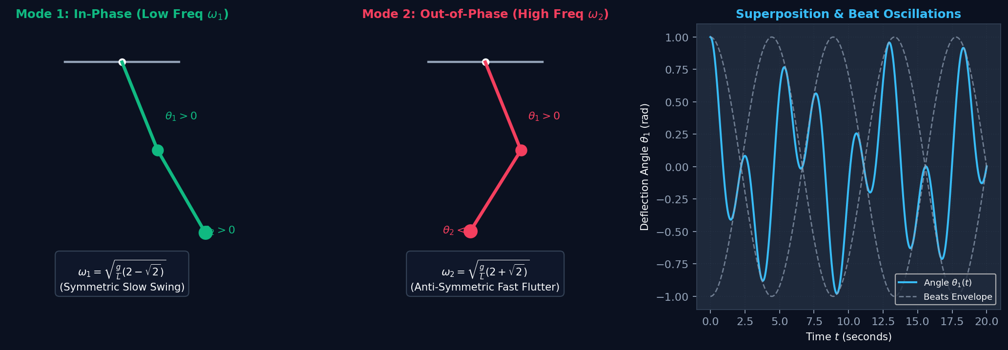
Before chaos emerges at large deflections, the small-angle regime ($|\theta_1|, |\theta_2| \ll 1$) reveals pure, elegant linear physics. The complex coupled system decouples into two independent normal modes of vibration with distinct characteristic frequencies $\omega_1$ and $\omega_2$.

Small-Angle Normal Modes and Beat Phenomenon in Double Pendulum

Figure 3.3.1: Small-angle normal modes: Mode 1 (In-Phase symmetric slow swing), Mode 2 (Out-of-Phase anti-symmetric fast flutter), and beat oscillation superposition.

1. Linearization of the Equations of Motion

For small angles $\theta_1, \theta_2 \ll 1$, we apply the Taylor approximations: $$\sin\theta \approx \theta, \qquad \cos(\theta_1 - \theta_2) \approx 1, \qquad \dot{\theta}_i^2 \approx 0$$ The nonlinear equations linearize into the classic coupled harmonic oscillator system:

$$(m_1 + m_2) L_1 \ddot{\theta}_1 + m_2 L_2 \ddot{\theta}_2 + (m_1 + m_2) g \theta_1 = 0$$ $$m_2 L_1 \ddot{\theta}_1 + m_2 L_2 \ddot{\theta}_2 + m_2 g \theta_2 = 0$$

2. Generalized Matrix Eigenvalue Problem

Assuming harmonic normal mode solutions $\theta_j(t) = A_j e^{i\omega t}$, we obtain the generalized eigenvalue problem:

$$\left[ \mathbf{K} - \omega^2 \mathbf{M} \right] \vec{A} = \mathbf{0}$$

where the symmetric mass and stiffness matrices are:

$$\mathbf{M} = \begin{pmatrix} (m_1 + m_2) L_1^2 & m_2 L_1 L_2 \\ m_2 L_1 L_2 & m_2 L_2^2 \end{pmatrix}, \qquad \mathbf{K} = \begin{pmatrix} (m_1 + m_2) g L_1 & 0 \\ 0 & m_2 g L_2 \end{pmatrix}$$

For equal masses ($m_1 = m_2 = m$) and equal lengths ($L_1 = L_2 = L$), the secular equation $\det(\mathbf{K} - \omega^2 \mathbf{M}) = 0$ simplifies to:

$$\omega^4 - 4\frac{g}{L} \omega^2 + 2\left(\frac{g}{L}\right)^2 = 0$$

Solving the bi-quadratic equation gives the exact normal frequencies:

$$\omega_1 = \sqrt{\frac{g}{L}(2 - \sqrt{2})} \approx 0.765 \sqrt{\frac{g}{L}}, \qquad \omega_2 = \sqrt{\frac{g}{L}(2 + \sqrt{2})} \approx 1.848 \sqrt{\frac{g}{L}}$$

3. Physical Interpretation of Normal Modes

• Mode 1 (Low Frequency $\omega_1$): The eigenvector ratio is $r_1 = \frac{\theta_2}{\theta_1} = +\sqrt{2} \approx +1.414$. Both rods swing in-phase in the same direction, resembling a flexible extended pendulum.
• Mode 2 (High Frequency $\omega_2$): The eigenvector ratio is $r_2 = \frac{\theta_2}{\theta_1} = -\sqrt{2} \approx -1.414$. The two rods swing out-of-phase in opposite directions, rapidly counter-balancing each other.
• Beats & Energy Transfer: In general superposition, energy oscillates back and forth between rod 1 and rod 2 at the beat frequency $\Delta\omega = \omega_2 - \omega_1$, creating envelope modulation!

Module 3.3 Small-Angle Normal Modes, Resonance & Harmonic Beats