Deterministic Chaos & The Butterfly Effect: Sensitivity to Initial Conditions
Interactive Physics Ready
Click "Run Code" to launch simulation and interactive parameter sliders.
Mathematical Problem Formulation
Theoretical Background & Explanation
Deterministic Chaos & The Butterfly Effect
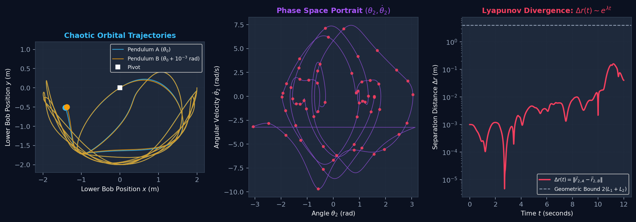
The concept of deterministic chaos implies that a physical system governed by completely exact, deterministic equations of motion without any stochastic randomness can nonetheless produce fundamentally unpredictable long-term trajectories due to exponential sensitivity to initial conditions.
1. The Maximal Lyapunov Exponent ($\lambda$)
Consider two initial states in 4D phase space $\vec{X}_A(0)$ and $\vec{X}_B(0)$ separated by an infinitesimal Euclidean perturbation $\|\Delta \vec{X}(0)\| = \delta_0 \ll 1$. In a chaotic dynamical system, the separation distance evolves exponentially in time:
The maximal Lyapunov exponent $\lambda$ is formally defined by the asymptotic limit:
• $\lambda < 0$: Regular dissipative system converging to a stable fixed-point attractor.
• $\lambda = 0$: Conservative, integrable periodic/quasi-periodic orbits (e.g. harmonic oscillators or planetary orbits without resonances).
• $\lambda > 0$: The system is chaotic. Adjacent trajectories diverge exponentially, destroying deterministic long-range forecastability!
2. The Predictability Horizon & Geometric Saturation
Because physical pendulums are mechanically bounded to a maximum possible distance $D_{\text{max}} = 2(L_1 + L_2)$, the exponential growth $\Delta r(t) \sim e^{\lambda t}$ cannot continue infinitely. It reaches a saturation boundary when the two bobs become as separated as physically possible in space:
Notice the logarithmic dependence: even if you improve your measurement precision by a factor of $1,000$ ($\Delta r_0 \to 10^{-3} \Delta r_0$), your forecast horizon $t_{\text{horizon}}$ only increases additively by $\frac{\ln(1000)}{\lambda} \approx \frac{6.9}{\lambda}$ seconds! This mathematical fact is why weather forecasting beyond two weeks is fundamentally impossible, as discovered by Edward Lorenz in 1963.
3. Energy Threshold: Transition from Integrability to Chaos
The double pendulum does not exhibit chaos at all energies:
• Low Energy Regime ($E < m_2 g L_1$): The potential well confines both angles to small amplitudes. KAM (Kolmogorov-Arnold-Moser) tori dominate phase space, and trajectories remain regular and quasi-periodic.
• Critical Transition ($E \approx m_2 g L_1$): The lower pendulum has sufficient energy to reach the inverted saddle point $\theta_2 = \pi$. Separatrix crossing creates homoclinic chaos.
• Fully Chaotic Regime ($E \gg m_2 g L_1$): KAM tori are shattered into a sea of chaos, and the phase space portrait exhibits ergodicity and dense orbital mixing.