Double Pendulum Simulation Studio
Interactive Physics Ready
Click "Run Code" to launch simulation and interactive parameter sliders.
Mathematical Problem Formulation
Theoretical Background & Explanation
Classical Mechanics: Double Pendulum Dynamics & Chaos
The double pendulum is the quintessential archetype of deterministic chaos in classical mechanics. While completely governed by deterministic Newton-Euler-Lagrange equations, its motion at moderate and high energies exhibits extreme sensitivity to initial conditions, complex fractal trajectories, and phase space mixing.
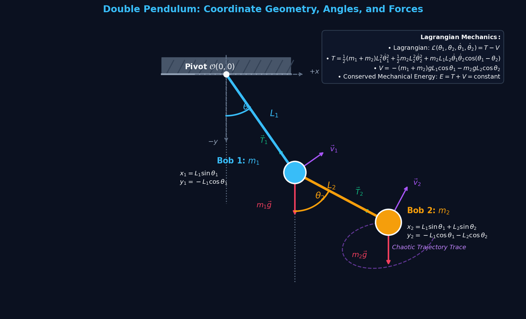
1. Coordinate Kinematics & Generalized Coordinates
Consider two point masses $m_1$ and $m_2$ suspended by rigid, massless rods of lengths $L_1$ and $L_2$ from a fixed frictionless pivot $\mathcal{O}(0, 0)$. Defining generalized coordinates $\theta_1$ and $\theta_2$ as the counter-clockwise deflection angles relative to the downward vertical:
Differentiating with respect to time $t$ yields the velocity components:
2. Kinetic & Potential Energy Formulation
The total kinetic energy $T$ of the two-particle system is:
Taking gravitational potential energy reference $V = 0$ at the downward equilibrium position ($\theta_1 = \theta_2 = 0$):
The Lagrangian function $\mathcal{L} = T - V$ fully defines the system's dynamics:
3. Euler-Lagrange Equations of Motion
Applying Hamilton's principle of stationary action $\frac{d}{dt}\left(\frac{\partial \mathcal{L}}{\partial \dot{\theta}_i}\right) - \frac{\partial \mathcal{L}}{\partial \theta_i} = -\gamma \dot{\theta}_i$:
Letting $\Delta = \theta_1 - \theta_2$, we rewrite the system in compact matrix form $\mathbf{M}(\vec{\theta}) \ddot{\vec{\theta}} = \vec{R}(\vec{\theta}, \dot{\vec{\theta}})$:
The determinant of the mass matrix is strictly positive for all physical parameters: $$\det \mathbf{M} = m_2 L_1 L_2 \left[ (m_1 + m_2) - m_2 \cos^2\Delta \right] = m_2 L_1 L_2 \left[ m_1 + m_2 \sin^2\Delta \right] > 0$$ By matrix inversion (Cramer's rule), the angular accelerations $\ddot{\theta}_1, \ddot{\theta}_2$ are computed unconditionally without singularities:
4. Numerical Runge-Kutta 4 (RK4) Integration & Conservation of Energy
The 2nd-order coupled ODEs are transformed into four 1st-order state equations for state vector $\vec{Y} = (\theta_1, \theta_2, \omega_1, \omega_2)^T$. The Runge-Kutta 4th Order (RK4) integration algorithm updates the state across time step $\Delta t$:
In the absence of damping ($\gamma = 0$), the total mechanical energy $E = T + V$ is a rigorous constant of motion ($dE/dt = 0$). The live simulation displays the energy breakdown and monitors energy conservation precision ($|\Delta E / E_0| < 0.05\%$).
5. Student-Friendly Parameter Tuning Guide
Use the live sliders below the workbench to explore exciting physics regimes:
• Small Angles ($|\theta_{1,2}| < 20^\circ$): Observe smooth, predictable, periodic/quasi-periodic normal mode oscillations.
• High Angles ($|\theta_{1,2}| > 90^\circ$): Witness the onset of deterministic chaos! The lower bob flips unpredictably over the top.
• Mass Dominance ($m_1 \gg m_2$ vs $m_1 \ll m_2$): When $m_1 \gg m_2$, the upper pendulum behaves almost as a simple pendulum driving the chaotic whip of $m_2$.
• Zero-Gravity ($g = 0$): Observe pure conservation of angular momentum and inertial tumbling!
• Damping ($\gamma > 0$): Watch the chaotic strange attractor collapse into the stable downward equilibrium sink $(0, 0)$.