Metric Tensor, Scale Factors & Christoffel Symbols Studio - Covariant vs Contravariant Bases in Curvilinear Coordinates
Interactive Physics Ready
Click "Run Code" to launch simulation and interactive parameter sliders.
Mathematical Problem Formulation
Theoretical Background & Explanation
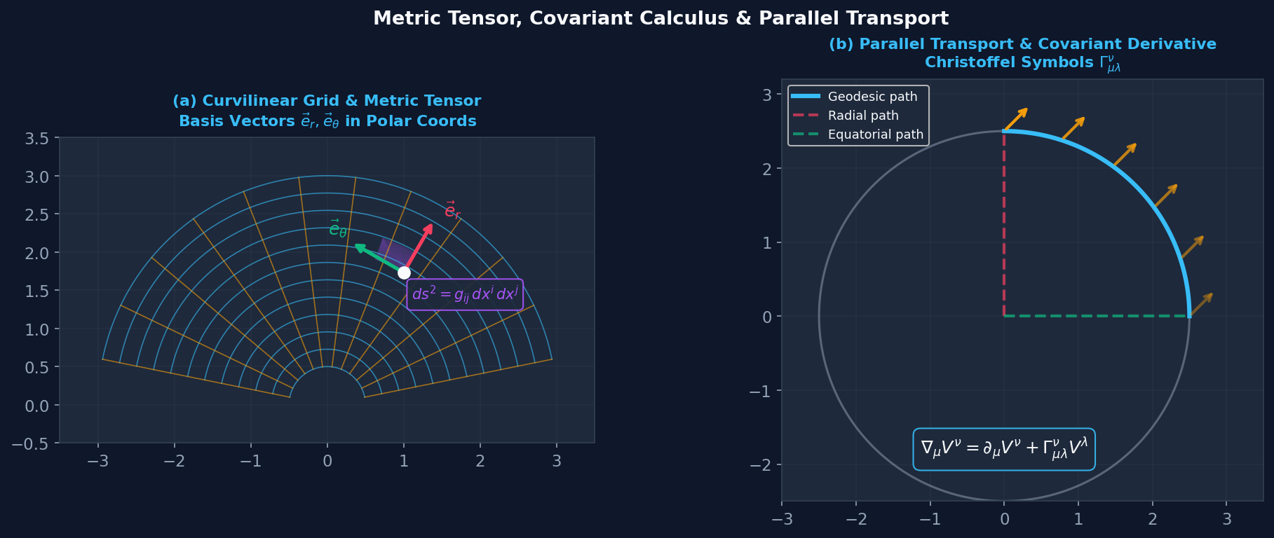
Figure 2.4: Metric Tensor & Differential Geometry: (a) Covariant metric $g_{ij}$ and basis vectors $\vec{e}_i = \partial \vec{r}/\partial u^i$, (b) Christoffel symbols $\Gamma^k_{ij}$ and parallel transport around a latitude circle showing holonomy deficit $\Delta\alpha = 2\pi(1 - \cos\theta_0)$.
The Metric Tensor $g_{ij}$
In any arbitrary curvilinear or Riemannian coordinate system $\{u^1, u^2, u^3\}$, the infinitesimal invariant distance $ds$ between two neighboring points is determined by the metric tensor $g_{ij}$: $$ds^2 = g_{ij} du^i du^j = g_{11}(du^1)^2 + g_{22}(du^2)^2 + g_{33}(du^3)^2 + 2g_{12}du^1 du^2 + \dots$$ The metric tensor acts as the "ruler" of spacetime, lowering indices ($v_i = g_{ij} v^j$) while its inverse $g^{ij}$ raises indices ($v^i = g^{ij} v_j$).
1. Covariant Basis Vectors & Scale Factors
For a position vector $\vec{r}(u^1, u^2, u^3)$, the tangent covariant basis vectors are $\vec{e}_i = \frac{\partial \vec{r}}{\partial u^i}$. The metric components are their mutual inner products:
In orthogonal curvilinear systems, $g_{ij} = 0$ for $i \neq j$. For example:
• Cylindrical $(r, \theta, z)$: $ds^2 = dr^2 + r^2 d\theta^2 + dz^2 \implies g_{rr} = 1, g_{\theta\theta} = r^2, g_{zz} = 1$.
• Spherical $(r, \theta, \phi)$: $ds^2 = dr^2 + r^2 d\theta^2 + r^2\sin^2\theta\, d\phi^2 \implies g_{rr} = 1, g_{\theta\theta} = r^2, g_{\phi\phi} = r^2\sin^2\theta$.
2. Christoffel Symbols of the Second Kind
Unlike Cartesian basis vectors, curvilinear basis vectors change their direction from point to point: $\frac{\partial \vec{e}_i}{\partial u^j} = \Gamma^k_{ij} \vec{e}_k$. The Christoffel symbols (affine connection coefficients) are completely determined by derivatives of the metric tensor:
Note: The Christoffel symbol $\Gamma^k_{ij}$ is symmetric in its lower indices ($\Gamma^k_{ij} = \Gamma^k_{ji}$ in torsion-free spaces), but is not a tensor itself!
3. Covariant Differentiation
Because the basis vectors vary spatially, the true directional derivative of a vector field (the covariant derivative $\nabla_j$) contains a correction term via $\Gamma$:
A curve $x^i(\lambda)$ is a geodesic (path of shortest proper distance) if its tangent vector is parallel-transported along itself: $$\frac{d^2 x^i}{d\lambda^2} + \Gamma^i_{jk}\frac{dx^j}{d\lambda}\frac{dx^k}{d\lambda} = 0$$
Physics Problem - Geodesics and Parallel Transport of Vectors on a Curved 2-Sphere (S^2) - Holonomy & Gauss-Bonnet
Interactive Physics Ready
Click "Run Code" to launch simulation and interactive parameter sliders.
Mathematical Problem Formulation
Theoretical Background & Explanation
Differential Geometry Problem: Holonomy Deficit on a Sphere
A key hallmark of intrinsic Riemannian curvature is that parallel transporting a vector along a closed circuit does not return the vector to its initial orientation. Consider a unit tangent vector parallel-transported around a constant latitude line $\theta = \theta_0$ on a 2-sphere $S^2$ of radius $R$. Derive the transport differential equation and determine the geometric angle (holonomy deficit $\Delta\alpha$) by which the vector is rotated upon completing one full loop.
1. Parallel Transport Equation on $S^2$
On a 2-sphere with metric $ds^2 = R^2 d\theta^2 + R^2\sin^2\theta\, d\phi^2$, the only non-zero Christoffel symbols are: $$\Gamma^\theta_{\phi\phi} = -\sin\theta\cos\theta, \qquad \Gamma^\phi_{\theta\phi} = \Gamma^\phi_{\phi\theta} = \cot\theta$$ Along a curve parameterized by longitude $\phi$, the parallel transport equation $\frac{D V^i}{d\phi} = 0$ reads:
2. Analytical Solution in Orthonormal Basis
Converting to normalized components in the orthonormal frame $\{\hat{e}_\theta, \hat{e}_\phi\}$: $$v_1 = R\, V^\theta, \qquad v_2 = R\sin\theta_0\, V^\phi$$ Differentiating yields simple harmonic rotational coupling:
3. The Gauss-Bonnet Theorem & Foucault Precession
Upon completing a full circuit $\Delta\phi = 2\pi$, the vector returns rotated by the holonomy deficit:
Profound Physical Connections:
• Gauss-Bonnet Theorem: The holonomy angle equals the integral of Gaussian curvature $K = 1/R^2$ over the enclosed spherical cap (the enclosed solid angle $\Omega$).
• Foucault Pendulum: A Foucault pendulum is a physical realization of parallel transport on Earth! In one sidereal day ($\Delta t = 24\text{ h}$), its plane of oscillation precesses by angle $\Delta\alpha = 2\pi\cos\theta_0 = 2\pi\sin(\text{latitude})$, taking $T = 24/\sin(\text{lat})$ hours to complete a revolution.
• Berry Phase: In quantum mechanics, adiabatic evolution of a quantum state around a closed parameter loop acquires an identical geometric Berry phase!