Module 1.3 Curl of Vector Fields & Circulation

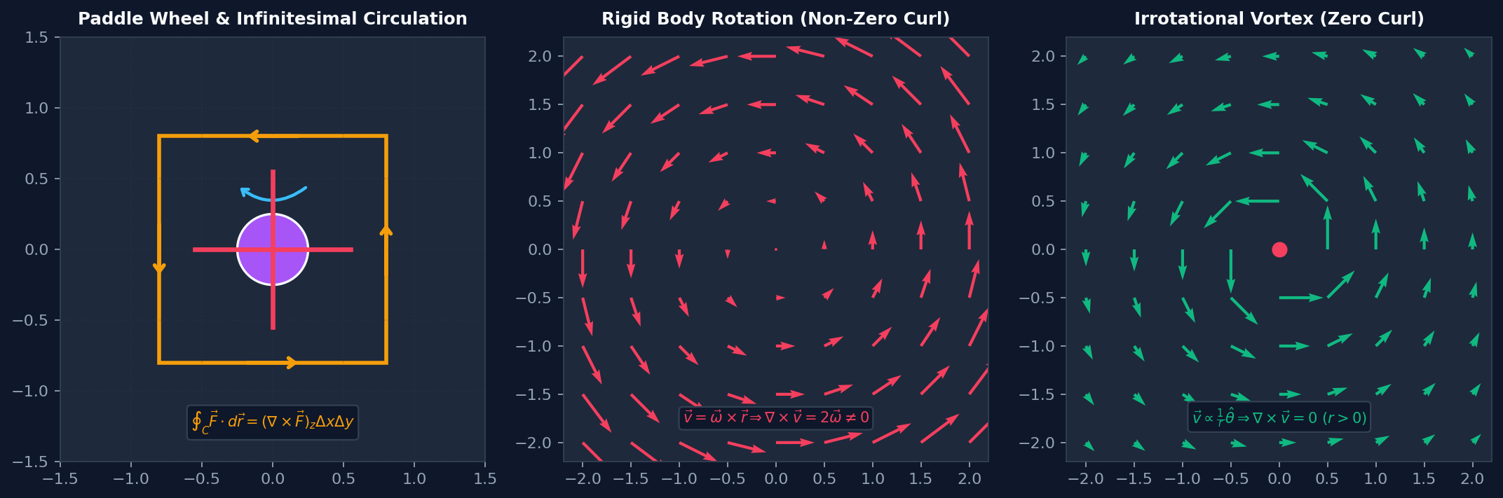
Figure 3.1: Conceptualizing Curl: (a) Infinitesimal circulation loop and paddle wheel rotation, (b) Solid-body rotation $\vec{v} = \vec{\omega}\times\vec{r}$ yielding non-zero uniform curl $\nabla\times\vec{v} = 2\vec{\omega}$, (c) Irrotational free vortex flow where fluid streamlines are circular but local curl is identically zero ($\nabla\times\vec{v} = 0$).

1. Cartesian Determinant Definition

2. The Paddle Wheel Thought Experiment

To develop an intuitive physical grasp of curl, imagine placing a microscopic paddle wheel with frictionless bearings at any test point in a fluid stream:
• If the paddle wheel rotates, the flow possesses local curl at that point, with induced angular velocity $\vec{\Omega}_{\text{wheel}} = \frac{1}{2}(\nabla \times \vec{v})$.
• If the paddle wheel does not rotate (even if moving along a circular path!), the local curl is zero.

3. Solid Body Rotation vs. Free Irrotational Vortex

A famous paradox in vector calculus contrasts two circular vector fields:
• Rigid Body Rotation ($\vec{v} = \vec{\omega} \times \vec{r} = -\omega y \hat{i} + \omega x \hat{j}$): $$(\nabla \times \vec{v})_z = \frac{\partial}{\partial x}(\omega x) - \frac{\partial}{\partial y}(-\omega y) = \omega - (-\omega) = 2\omega \neq 0$$ Every fluid element rotates about its own centroid with angular velocity $\omega$.
• Irrotational Free Vortex ($\vec{v} = \frac{\Gamma}{2\pi r} \hat{\theta} = \frac{\Gamma}{2\pi} \frac{-y\hat{i} + x\hat{j}}{x^2 + y^2}$): $$(\nabla \times \vec{v})_z = \frac{\Gamma}{2\pi} \left[ \frac{\partial}{\partial x}\left(\frac{x}{x^2+y^2}\right) - \frac{\partial}{\partial y}\left(\frac{-y}{x^2+y^2}\right) \right] = 0 \quad (\forall r > 0)$$ Even though the streamlines are concentric circles, the speed scales as $1/r$. The outer edge of a test paddle moves slower than the inner edge by just the right amount to keep the paddle wheel pointing in a constant direction without rotating!

4. Irrotational Vector Fields & Scalar Potentials

Because the curl of any gradient is identically zero ($\nabla \times (\nabla \phi) \equiv \vec{0}$), any curl-free vector field can be expressed as the gradient of a single scalar potential $\phi$. Examples include electrostatic fields ($\nabla \times \vec{E} = \vec{0} \implies \vec{E} = -\nabla V$) and Newtonian gravitational fields.

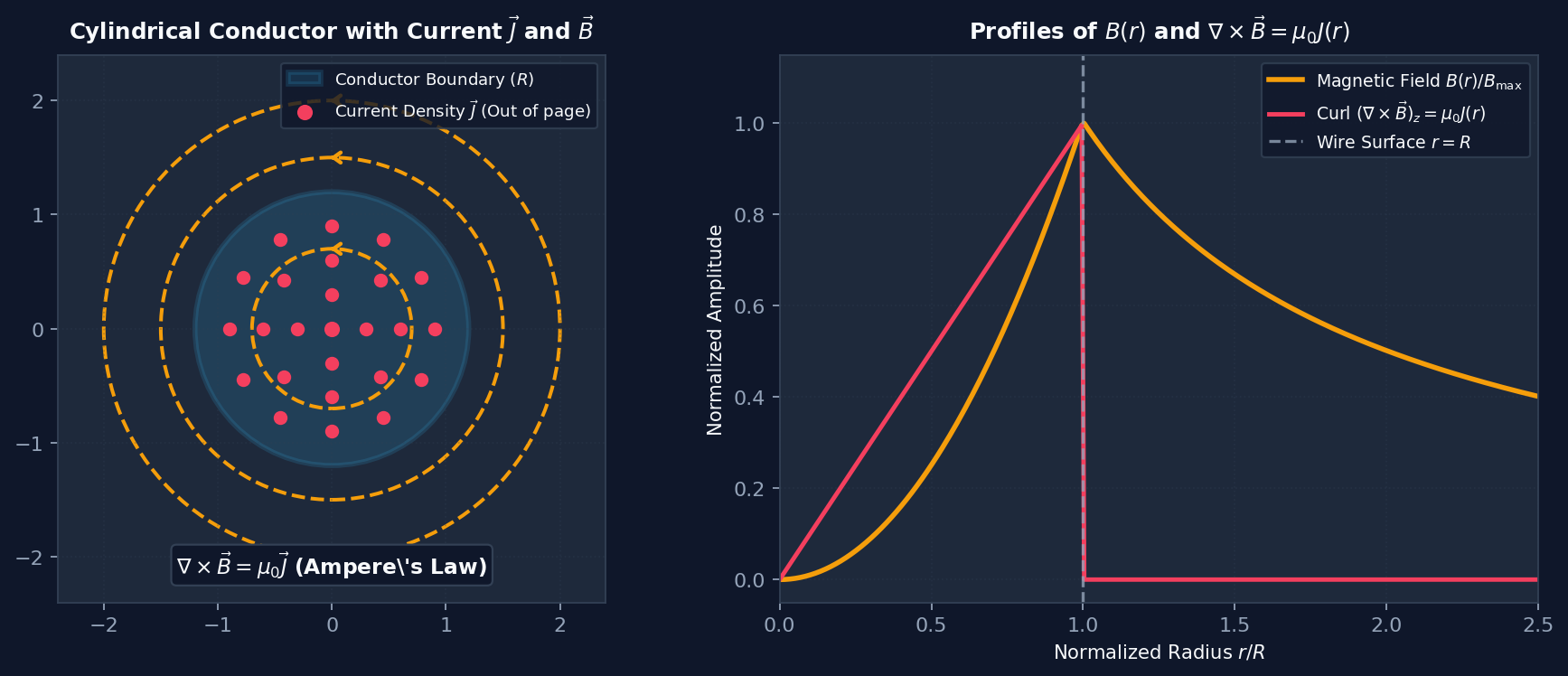
Figure 3.2: Ampere's Circuital Law & Magnetic Curl: (Left) Cylindrical conductor cross-section with non-uniform current density $J(r)$ and concentric magnetic field loops $\vec{B}$, (Right) Radial profiles showing $B(r)$ rising inside the wire, peaking at $r=R$, and decaying as $1/r$ outside where $\nabla \times \vec{B} = 0$.

1. Total Current Integration

Integrating the current density across concentric circular rings of area $dA = 2\pi r dr$:

2. Magnetic Field Calculation

Due to axial and azimuthal symmetry, the magnetic field is purely azimuthal: $\vec{B} = B(r)\hat{\theta}$. Applying Ampere's law along a circular loop of radius $r$: $$\oint_C \vec{B} \cdot d\vec{r} = B(r) \cdot 2\pi r = \mu_0 I_{\text{enc}}(r)$$
• Inside the Wire ($r \le R$):

• Outside the Wire ($r > R$): $$B_{\text{out}}(r) = \frac{\mu_0 I_{\text{tot}}}{2\pi r} = \frac{\mu_0 J_0 R^2}{(n + 2) r}$$

3. Cylindrical Curl Verification

In cylindrical coordinates $(r, \theta, z)$, the $z$-component of curl is:

Substituting $B_{\text{in}}(r)$: $$(\nabla \times \vec{B})_z = \frac{1}{r} \frac{d}{dr} \left[ \frac{\mu_0 J_0}{(n+2)R^n} r^{n+2} \right] = \frac{1}{r} \left[ \frac{\mu_0 J_0 (n+2)}{(n+2)R^n} r^{n+1} \right] = \mu_0 J_0 \left(\frac{r}{R}\right)^n = \mu_0 J(r)$$ For $r > R$, since $r B_{\text{out}}(r) = \text{constant}$, the derivative is identically zero: $\nabla \times \vec{B} = \vec{0}$.